Quantification of urban heat islands using automatic weather station data and smart-city networks

1. Introduction

Population increases in large cities have triggered a rapid expansion of urban areas along with increases in density, and these changes are affecting multiple aspects of urban environments (He et al., 2021; Li et al., 2020; Wang et al., 2020; Xu et al., 2009). Urban heat islands (UHIs) exemplify such environmental changes caused by urbanisation (Arshad et al., 2021; Ramírez-Aguilar and Souza, 2019). The UHI is a phenomenon wherein the temperature in urban areas increases above that of the surrounding environment (Morini et al., 2018). This can be attributed to the remarkably high proportion of the anthropogenic land-cover materials, such as concrete and asphalt, used in urban construction. These materials demonstrate lower albedo compared to natural green areas and absorb increased solar radiations. This results in the accumulation of heat energy on the ground surface. Moreover, unlike natural areas, these materials afford zero water retention and permeation functions, and moisture evaporation from the underlying soil is blocked, and this causes the surrounding atmosphere to become dry (Carlson, 2007; Erell et al., 2012; Morabito et al., 2021; Spronken-Smith et al., 2000). A long-lasting UHI and corresponding heat wave can potentially cause an increase in the mortality rate. The persistent global warming and high-density urban development are exacerbating such events. The aforementioned adverse effects of UHIs can be mitigated through attainment of spatial solutions. Specific diagnosis and mitigation information concerning heat islands is required to this end.

Although several studies have investigated UHIs from different perspectives and identified their underlying causes (Arshad et al., 2021; Bartesaghi-Koc et al., 2020; Ramírez-Aguilar and Souza, 2019). The results obtained in these studies can be discussed differently depending on the method used to acquire the temperature data. The temperatures that define heat islands can be studied considering the land surface or atmosphere, and these two data types possess different characteristics (Bartesaghi-Koc et al., 2020). Notably, studies concerning the surface urban heat island (SUHI) performed using satellite imagery obtained via remote sensing are less affected by external conditions and can produce uniform measurement values for the intended target site without spatial constraints. By exploiting this method, a variety of research can be conducted through the calculation of spectral indices related to land use, such as the Normalised Difference Vegetation Index (NDVI), which is useful for indirect measurements of the presence and density of plants, and the Normalised Difference Built-up Index (NDBI); spatiotemporal patterns of land surface temperatures (LSTs) can also be studied easily over a wide area (Chen et al., 2014; Du et al., 2016; Morabito et al., 2021; Santamouris, 2014). The method that uses satellite imagery represents an indirect assessment of the heat-island phenomenon (Gallo et al., 2011), and thus, it is limited in that it cannot be used to reconstruct the air temperature characteristics actually experienced by residents directly.

Research on UHIs based on atmospheric temperatures is conducted by measuring the temperature and other meteorological variables, such as the wind speed and humidity, which influence how humans perceive heat. The characteristics of the required data vary depending on whether the heat island is a boundary-layer urban heat island (BLUHI) or a canopy-layer urban heat island (CLUHI). A BLUHI is a heat island that can be explained based on meteorological phenomena at the mesoscale or city scale, and regional differences such as differences between urban and rural areas are typically discussed. Therefore, the method for measuring a BLUHI relies on the temperature at which sufficient convection has occurred without being affected by radiant heat, and these data are measured on high buildings or by installing sufficiently high weather towers (Parsaee et al., 2019). A CLUHI is a heat island measured by using temperatures within the lower parts of a city and represents a microclimate affected by surrounding land uses, street canyon structures, and so forth. Therefore, the temperatures of canyons and all spaces below the rooftop level inside the city are measured and used (Parsaee et al., 2019). In other words, it requires a measurement network with a higher spatial resolution than the measurement network used for a BLUHI. Furthermore, there are some notable constraints, namely, hour-long measurements need to be acquired, non-instantaneous temperatures are required for error filtering of the temperatures, and a specific temperature has to be measured under the condition that there is no urban element (e.g., vehicles and pedestrians) affecting the surroundings (Mirzaei and Haghighat, 2010).

Several extant studies have used the temperature-monitoring network built by a state and/or local governments to investigate BLUHIs; whereas other investigations have involved the measurement of canopy-layer temperatures (Park et al., 2017; Park et al., 2019). However, these studies have encountered several limitations, including the unavailability of data to simultaneously compare different locations owing to physical and cost constraints, insufficient measurement samples, and lack of monitoring networks that cover the entire city (Mirzaei and Haghighat, 2010). Although few studies have considered the use interpolation methods to overcome these limitations (Bhowmik and Costa, 2015; Jahangir and Moghim, 2019; Liu et al., 2017; Sánchez et al., 2003; Shtiliyanova et al., 2017; Yadav and Sharma, 2018), there remains the limitation in that the results obtained do not reflect the actual measurement values for the entire city. Instead, they correspond to values obtained via statistical estimation. To overcome this problem and facilitate the acquisition of high-spatial-resolution urban climate data, the state and local governments in several countries are considering the development of high-resolution air temperature monitoring networks or collaborating with private sector companies and/or citizens to develop such networks. These data can be used to examine UHIs and can be used to perform canopy layer measurements.

This study aims was to compare the high-resolution temperature data (Smart Seoul Data of Things; S-DoT) and mesoscale national monitoring network data (Automatic Weather Station; AWS) used in conventional studies to analyse the difference in the temperature characteristics between the two spatial resolutions and evaluate the temperature-influencing factors. Furthermore, the interpolated temperatures and high-resolution temperature data are compared to discuss the canopy and boundary layer characteristics.

2. Materials and methods

2.1. Overall study approach

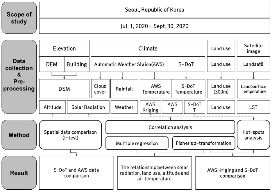
The metropolitan region of Seoul, the capital city of Korea, was considered in the analysis performed in this city. The city government of Seoul has developed several systems to facilitate the collection and analysis of data pertaining to urban phenomena across neighbourhoods. Among these, the Smart Seoul Data of Things (S-DoT) was deployed under a pilot program in 2019, the data obtained as part of which was publicly released in April 2020. This study was performed over the period between July 1, 2020 and September 30, 2020, i.e., the summer months. Fig. 1 presents a flowchart of the tasks performed in this study. First, the data required for analysis were first collected and pre-processed. Next, the temperatures obtained using S-DoT and AWS were compared via spatial statistical analyses, and their corresponding relationships with the solar radiation (SR), green-area ratio (GAR), and altitude were evaluated. Subsequently, the interpolation results obtained using AWS and S-DoT were comparatively examined. Each variable was selected to reflect land use, altitude, and urban structural factors that have been discussed as possible causes of temperature differences between the two observation networks (Park, 2021). For land use, GAR was selected as a variable to figure out differences in green space, and SR was used to reflect urban structural factors. Altitude has a significant impact on air temperature (Choi, 2011; Yim & Lee, 2017), so we used it to reflect factors related to differences in altitude within location.

Fig. 1.

Flowchart of proposed study

2.2. Data collection and pre-processing

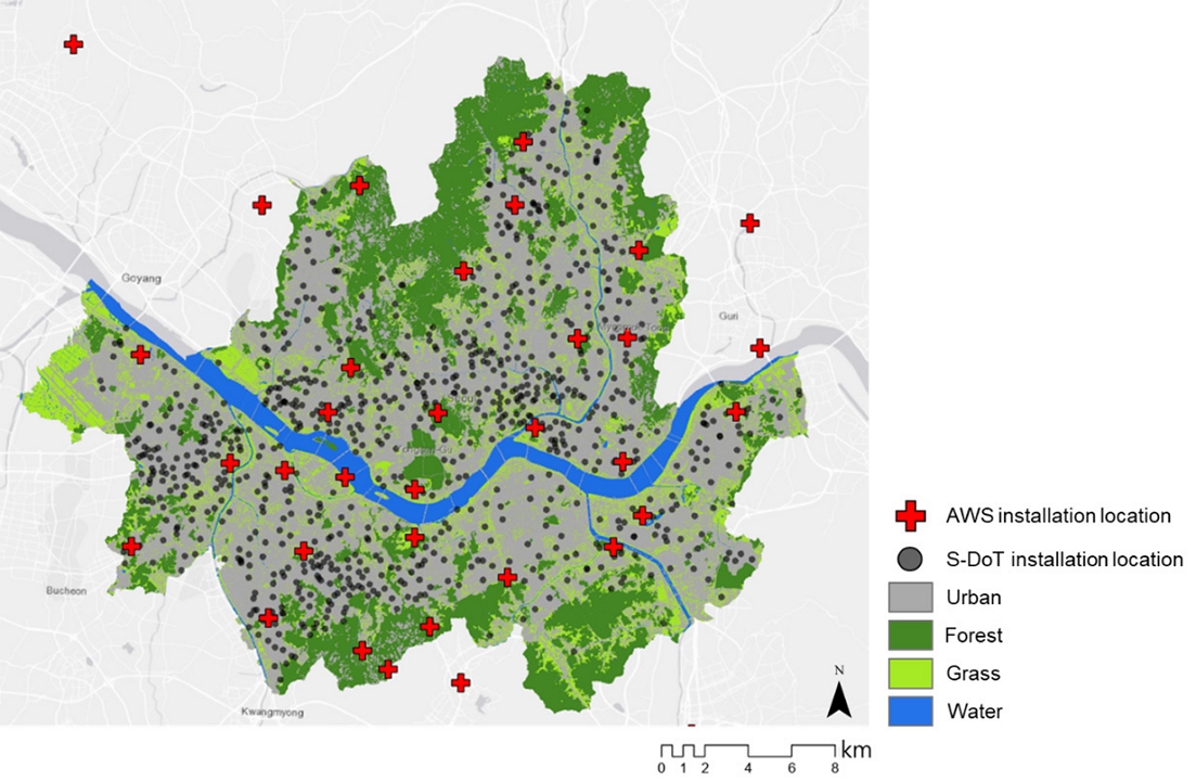
The elevation, climate, land use, and satellite image data were collected and pre-processed. Elevation data were used to build a digital surface model (DSM), and the daily solar radiation (SR), which was corrected based on cloud cover, was calculated. The weather data were obtained from the S-DoT, a high-resolution temperature-monitoring network of Seoul, and the AWS system operated by the government was used as a reference temperature-monitoring network. Those stations were installed throughout Seoul, and each installation location is shown in Fig. 3. The interpolated data of the AWS were generated by using the daily temperature data of the AWS. Subsequently, the land-cover ratios around the weather stations were calculated, and the LSTs were calculated by using the Landsat 8 satellite images.

2.2.1. High-resolution air temperature data for Seoul (S-DoT)

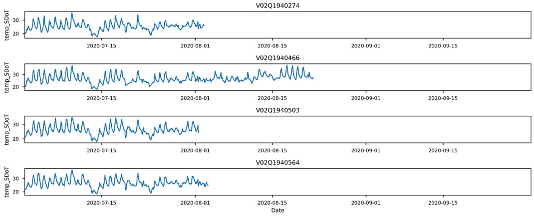
S-DoT is a group of monitoring sensors that collect urban data generated in the city of Seoul. In total, 850 units have been installed across Seoul (as of 2020. S-DoT sensors are mainly installed on closed-circuit TV supporting plates, telephone poles, and exterior walls of buildings). With the S-DoT, hourly measurement information on 10 types of data (air temperature, humidity, illuminance, noise level, particulate matter including PM10 and PM2.5, ultraviolet (UV) rays, vibrations, number of visitors, wind direction, and wind speed) is collected. In this study, only the data from 8:00 to 20:00 on the observation date were used, and S-DoT points were excluded when errors were found in the data (Fig. 2).

Fig. 2.

S-dot data with observational errors removed

2.2.2. National temperature data from the Automatic Weather System

The AWS is a terrestrial observation system that has been in operation since 1997 by the Korea Meteorological Administration (KMA). Monitoring stations are installed at 504 locations nationwide, and these automatically monitor the air temperature, wind, precipitation, humidity, and air pressure. As of 2020, there were 27 monitoring stations in Seoul. If nearby stations were included, there were 33 monitoring stations with data available. The AWS air temperature sensors are installed at a height of 1.2–2.0 m above the ground and in places where a ventilation wind speed of 2.5–10 m/s is maintained. The AWS constructs 1-min data by averaging six data points sampled at 10-s intervals at the measurement point. The hourly air temperature dataset was constructed by averaging 1-min data in units of an hour, and the air temperature data were recorded in units of 0.1°C (KMA, 2019).

Fig. 3.

Locations of S-DoT and AWS installations in Seoul

2.2.3. Land cover around the monitoring stations (S-DoT and AWS)

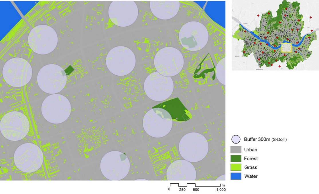
A spatial statistical analysis was performed to investigate the relationship between the air temperature difference and land-use characteristics of the two types of monitoring stations (S-DoT and AWS). For the data used for land use, land-use maps created by the Ministry of Environment were used, and the land-use data were divided into seven categories (urban, agriculture, forest, grass, wet land, and water). Among the land uses, forest, grass, wet land, and water were defined as green areas and analysed accordingly. Agricultural land in Seoul was excluded from green areas because most of the land refers to greenhouses. For land-use characteristics around the S-DoT sites, the land-use ratio was calculated by using buffer information within a 300 m circle around the centre of the S-DoT site (Fig. 4).

Fig. 4.

Method for determining land-use characteristics around S-DoT sites

2.2.4. Solar radiation

The SR energy-calculation model developed by Fu and Rich (2002), which in turn, is based on the algorithm developed by Rich et al.(1994), was used in this study. This model derives the SR levels by repeatedly calculating the direct and diffused radiation at all locations on the topographic surface. Elevation information is required as input data for the calculation of SR energy, but because the digital elevation model (DEM) only reflects the elevation of the ground surface, the radiation generated by the buildings is not included (Wang et al., 2016). Therefore, a digital surface model (DSM) was developed and used in this study. The Integrated Building Information of Seoul was used to build the information needed for this study, and the DSM was developed by assuming a height of 3 m from the top floor. SR was calculated based on the completed DSM.

The SR for cloudy days was calculated by using the SR adjustment formula depending on the cloud cover (Kasten and Czeplak, 1980; Nersesian, 2018), and KMA data were used for the cloud cover information.

$\[ P={990}^{\mathrm{*}}\left(1-{0.75}^{\mathrm{*}}{F}^{3.4}\right) \]$

(1)

• where P represents the SR and F represents the cloud cover.

2.2.5. AWS interpolation (kriging)

The AWS-based temperature information was created by using ordinary kriging among the interpolation methods (“AWS kriging” hereinafter) to estimate the information for S-DoT points by spatialising the limited temperature information of AWS. Interpolation is a method of estimating the information for a point where there are no observation values, and this is accomplished based on a limited number of observations made elsewhere. In fact, kriging has been used to investigate the temperature or UHI characteristics of points without the need for weather stations (Bhowmik and Costa, 2015; Jahangir and Moghim, 2019; Liu et al., 2017; Sánchez et al., 2003; Shtiliyanova et al., 2017; Yadav and Sharma, 2018). Kriging is a topographic statistical interpolation method that performs predictions by assigning weights to the observation values of the surroundings based on a statistical model. It differs from inverse distance weighting (IDW), a typically used interpolation method, in that the method of applying the weights is different. In IDW, weights are determined by the distance from the observation points, but in kriging, the concept of autocorrelation is applied to the correlation strength between the observation points when the weights are determined (ESRI online).

2.3. Methods

First, the daily mean temperatures were compared between the S-DoT and AWS. The statistical difference in mean temperatures between the monitoring stations was validated using a t-test. We then checked whether there was a difference in temperature depending on the spatial distribution. The AWS temperature and mean temperature of the S-DoT distributed within 300 m of the AWS site were statistically compared to check if the spatial distributions were different. In addition, we compared the temperature differences between the monitoring stations located in forests and the city centre.

Next, the correlations between the temperature and three factors, namely, the SR, GAR, and altitude were analysed in two steps. In the first step, it was assumed that the rainy and sunny days would show different correlations, and all of the data were grouped into either rainy or sunny days, after which their correlations were analysed. In the second step, by using daily data from sunny days, we investigated the explanatory power of each model derived through a multilinear regression analysis of the AWA–S-DoT data. Here, the input data of the S-DoT were sorted and broken into 150 equal-sized quantiles based on the dependent variable for 850 monitoring stations to conduct the analysis (Pan et al., 2018).

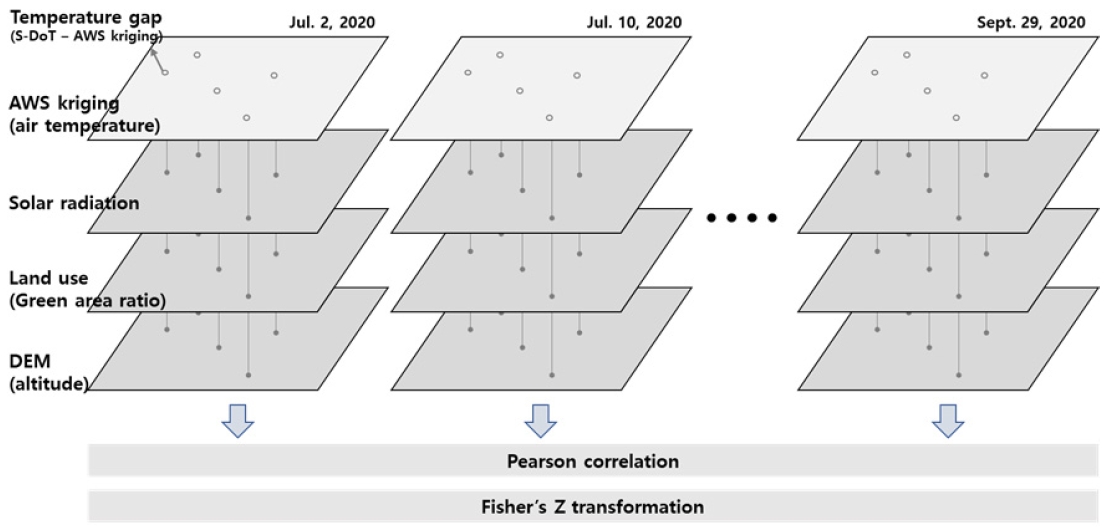
Finally, the statistical difference between the AWS kriging and S-DoT temperatures at the installation locations of the S-DoT (n = 850) was analysed to determine the difference between the kriging data and the city monitoring data. Then, correlations between the temperature and the three factors (SR, GAR, and altitude) were analysed for each day (sunny days) to analyse which factors were correlated with the difference between the two datasets. The correlation coefficients were comparatively analysed using Fisher’s Z transformation (Fisher, 1921) to compare the daily correlations. As depicted in Fig. 5, the analysis was performed by generating separate installation locations for S-DoT and daily data sets.

Fig. 5.

Comparison of correlations between air temperature (AWS kriging, difference between AWS kriging and S-DoT) and factors of interest (SR, GAR, and altitude)

3. Results

3.1. Temperature distribution of S-DoT and AWS

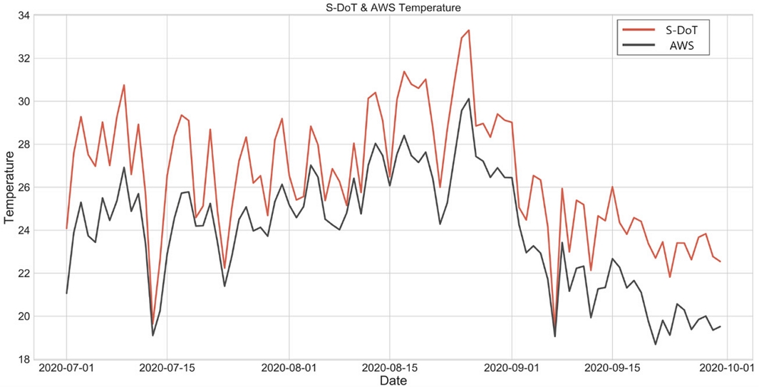
In the results of the daily distribution comparison between the two datasets from the S-DoT and AWS, both monitoring station types showed similar patterns for the daily mean temperature at all monitoring stations (Fig. 6). The mean temperature obtained using S-DoT equalled 26.51°C in summer, whereas that obtained using AWS was 23.93°C. Accordingly, the mean S-DoT temperature equalled 2.58°C higher compared to its AWS counterpart. Furthermore, the standard deviation of the S-DoT data was greater than that of the AWS data, whereby the mean variation of the S-DoT data (7.3%) was higher than that of the AWS data (5.1%). In addition, the t-test results for the difference between the two monitoring station types showed that a statistically significant difference existed between the mean temperatures of the S-DoT and AWS. On a day-to-day basis, the difference between temperatures measured using S-DoT and AWS revealed the S-DoT temperature to exceed the corresponding AWS value by 2.54°C on average. The corresponding difference in the standard deviations equalled 1.02.

Fig. 6.

Daily S-DoT air temperatures and AWS data

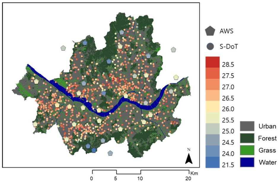
In the comparison of the mean temperatures of the S-DoT and AWS according to the monitoring point, the mean was statistically different between the two datasets (t-statistic = -12.489, p-value = 0.000) (Table 1). Furthermore, the AWS tended to show lower temperatures than the S-DoT within 300 m. The air temperatures measured by the AWS located near the forests (n = 19, mean = 24.5°C) were generally lower than those of the AWS located in the urban areas (n = 12, mean = 25.2°C), and the temperature distribution range of the monitoring stations was smaller for the AWS than for the S-DoT (Fig. 7). Specifically, the temperature range of AWS equalled 23.35–25.36°C (i.e., 2.01°C) while that of S-DoT equalled 24.01–28.37°C (i.e., 4.36°C).

Table 1.

Results for the paired sample tests

Fig. 7.

Spatial distribution of mean air temperatures (S-DoT versus AWS)

3.2. Relationship between SR, land use, altitude, and air temperature

3.2.1. Correlation analysis of each factor for all data

In the analysis results for the correlations between the air temperature and the three factors (SR, GAR, and altitude) within the S-DoT and AWS data, the temperature had a positive (+) relationship with the SR, whereas the temperature had negative (-) relationships with the GAR and altitude, regardless of rainfall. In the analysis results for all of the days, the AWS showed a positive correlation of 0.364 with the SR, while it showed negative correlations of -0.113 and -0.145 with the GAR and altitude, respectively. Meanwhile, for the S-DoT, the correlation coefficients were 0.486, -0.090, and -0.079 for the SR, GAR, and altitude, respectively. These correlations were different between the rainy and sunny days, and the air temperature had a stronger correlation with the SR on sunny days. The AWS results showed an approximately 0.274 higher positive correlation on sunny days, and the S-DoT results showed a positive correlation of approximately 0.171. The GAR showed a difference of 0.1 for both the AWS and S-DoT, and the altitude showed differences of 0.17 and 0.06, respectively.

Table 2.

Correlation between the air temperature and factors of interest (SR, GAR, altitude) according to the weather (sunny and rainy conditions)

3.2.2. Factor analysis using the regression equation for daily data (explanatory power %, weight for each variable)

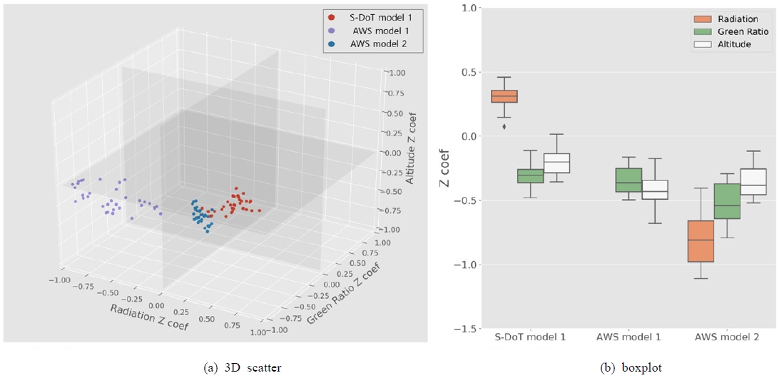
In the results of the multilinear regression analysis conducted for sunny days using the daily data in the S-DoT and AWS datasets, the S-DoT Model 1 showed that the air temperature had a positive relationship with the radiation (mean of β = 0.306), and negative relationships were found for the GAR (mean of β = -0.314) and altitude (mean of β = -0.205). The average explanatory power was 34.4%, and the ratios of dates with a p-value of 0.05 or less were equal to 94.1% for the radiation and GAR and 70.6% for the altitude.

Table 3.

Regression analysis results obtained daily data

In AWS Model 1, the air temperature had a negative relationship with all three factors including the radiation (mean β = -0.524), GAR (β = -0.351), and altitude (β = -0.805). The average explanatory power was 51.9%, and the ratios of the dates with a p-value of 0.05 or less were 73.5% for radiation, 69.6% for GAR, and 97.0% for altitude. In AWS Model 2, the air temperature had a negative relationship with the GAR (mean of β = -0.225) and altitude (mean of β = -0.753). The temperature of the AWS was significantly affected by altitude. The average explanatory power of the regression model was 70.8%, and the ratios of the dates with a p-value of 0.05 or less for each variable were 61.8% for the GAR and 100% for the altitude.

The observed deviations in the standardised coefficients of the multilinear regression analysis by date were found to differ across models. In S-DoT Model 1, the standard deviation equalled less than 0.1 for SR (std. dev. of β = 0.091), GAR (std. dev. of β = 0.092), and altitude (std. dev. of β = 0.099). Meanwhile, the AWS Model 1 demonstrated the largest deviations with respect to SR (std. dev. of β = 0.200), GAR (std. dev. of β = 0.149), and altitude (std. dev. of β = 0.121) among the three models. In AWS Model 2, the standard deviation by variable equalled 0.100 for GAR and 0.132 for altitude. As shown in Fig. 8, the beta coefficients of S-DoT Model 1 and AWS Model 2 were concentrated, while those of AWS Model 1 were scattered.

Fig. 8.

Distribution of beta coefficients for three models considered in this study

3.3. Comparison between AWS kriging and S-DoT data

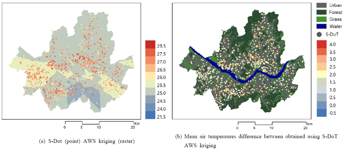
The data obtained from the AWS by kriging (AWS kriging) were compared to the temperature distribution of the S-DoT. The mean value of AWS kriging equalled 24.80°C, which differed the corresponding mean obtained using S-DoT by 1.72°C. In other words, AWS kriging revealed AWS temperatures to be were generally compared to their S-DoT counterparts. Furthermore, the standard deviation of AWS kriging was 0.20, whereas that of the S-DoT was 0.51, which was indicative of a narrower distribution. We compared the spatial temperature difference between the two monitoring station types and confirmed that the temperature difference decreased when the monitoring point was near (200 m) the forest area (Fig. 9). The mean temperature equalled 1.43°C for the monitoring points located near the forest area; in other regions, this mean temperature equalled 1.82°C.

Fig. 9.

Spatial distributions of mean air temperatures

By analysing the changes in the AWS interpolation (kriging) temperatures of S-DoT points and SR, GAR, as well as altitude, this study confirms the absence of a radiation correlation with the above-mentioned parameters. Although the GAR revealed a weak negative correlation (-0.155), the same was statistically insignificant on 44.1% of the days. The altitude demonstrated a strong negative correlation (-0.657), which was statistically significant on all days. In contrast, the temperature difference between the S-DoT and AWS kriging was statistically significant on all days, as revealed by the results of the correlation analysis for SR (83.7%), GAR (100%), and altitude (98.9%). The mean Fisher’s Z value equalled 0.409 for SR, which indicates a positive correlation, whereas equalled -0.805 for GAR—i.e., a negative correlation. The altitude, too, demonstrated a negative correlation of -0.619.

Table 4.

Mean Fisher’s Z transformation values for air temperatures obtained via AWS kriging as well as temperature difference between S-DoT and AWS kriging and factors of interest SR, GAR, and altitude

4. Discussion

4.2. Air temperature according to BLUHI, CLUHI, and SUHI

The measuring method and characteristics of heat islands vary depending on the measurement method used for air temperature. The BLUHI approach measures the heat-island phenomenon while focusing on the city centre at a mesoscale. This measurement method characteristically assumes the atmosphere in the upper part of the city to represent a heat island, and some studies have noted that it is desirable to measure the temperature at the top of the highest buildings and to install the monitoring devices at locations that are not affected by the surrounding buildings (Branea et al., 2016). The CLUHI approach focuses on heat islands at a more local scale and requires more detailed high-resolution data than the BLUHI approach. On such a local scale, there is a high possibility of reflecting radiation (Nakamura and Mahrt, 2005). Park (2021), who compared S-DoT with AWS and ASOS, discussed that the difference in temperature between the two stations may be due to the height of the station installation. In addition, the S-DoT is installed on closed-circuit TV camera mounting plates, building exterior walls, and so forth, and as a result, it likely reflects the radiation depending on the installation location, which may be a result of the influence of artificial heat generated in cities such as buildings, roads, outdoor air conditioner units, etc (Park, 2021). In other words, the AWS is a mesoscale-monitoring network that measures a BLUHI and the S-DoT is a microscale-monitoring network that measures a CLUHI. Therefore, even if the same temperature is observed, S-DoT is an urban environment that reflects artificial heat and is measured at a lower height, while AWS is measured at a higher location, resulting in different characteristics.

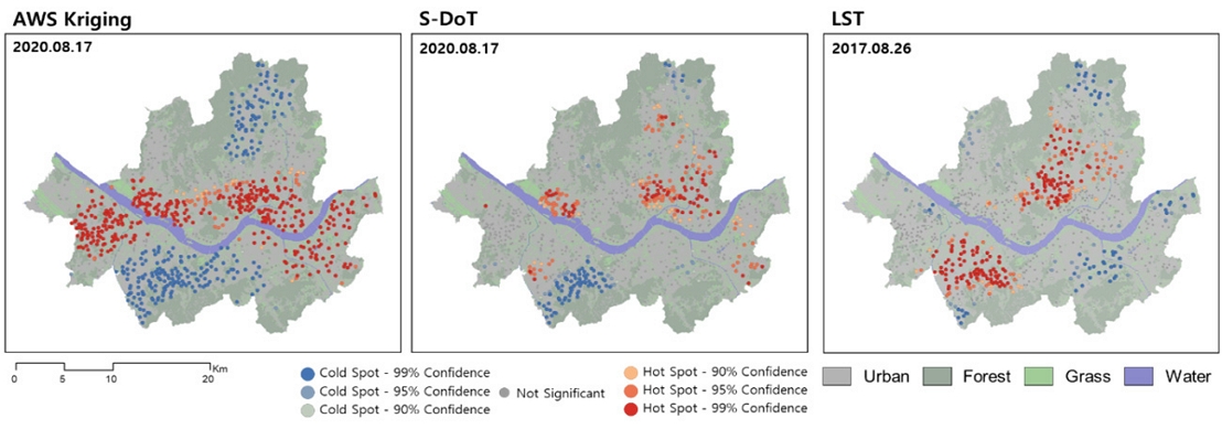
Even if the same heat island is investigated, the results will be different depending on which data are used (i.e., air temperature or surface temperature data) (Fig. 10, which compares results obtained at three data points). This confirms that the heat-island hot spots in the investigated area appear differently depending on which data—AWS kriging (mesoscale), S-DoT (microscale), and LST (surface temperature)—are used. The results obtained considering the AWS kriging and S-DoT data revealed different hot-spot-distribution ranges. The S-DoT showed local hot spots, whereas the AWS kriging showed a global distribution. The LST results also showed local hot spots similar to those of the S-DoT, but the spatial distribution was different because the characteristics of surface temperature and air temperature are different from each other (Branea et al., 2016; Sheng et al., 2017). In brief, the type of heat island discussed will differ depending on the scale of the spatial solution, and the characteristics of the data required would differ as well. So, not only are the heat island regions different depending on the data used, but the features that need to be discussed are also different. Therefore, when discussing spatial solutions, it is important to consider the data used and the scale.

Fig. 10.

Spatial air-temperature hotspots identified using AWS kriging, S-DoT, and LST

When the results of the interpolation at the mesoscale (AWS kriging) and the results of the microscale (S-DoT) were compared, a temperature difference was found. This difference seems to be a result of the aggregation of urban microclimates due to the low density of temperature-monitoring stations, whereby the heat and artificial heat were reflected according to the structure of urban buildings in the process of aggregation (Petralli et al., 2014). The canopy-layer temperature cannot be accurately determined via numerical interpolation owing to the difficulty involved in incorporating complex urban structures (Asdrubali and Desideri, 2019). In fact, the difference between the canopy- and boundary-layer temperatures increases with increase in the urbanisation ratio around monitoring stations and decrease in GAR. In urban areas, the difference between the said temperatures increases owing to the heat generated by the buildings and roads (Sailor 2013), and it decreases with increase in GAR owing to the heat-island reduction effect of green areas that reduce anthropogenic heat (Jin et al., 2011; Li et al., 2011; Yuan and Bauer, 2007). The radiation appears differently depending on the city structure, and this difference seems to affect the S-DoT results, wherein the microclimate is determined at the street level (Zhu et al., 2020). In contrast, as these differences are aggregated in AWS kriging, the difference between the S-DoT- and AWS-kriging-based temperatures increases as the radiation increases. In the case of altitude, because the target study areas were at high altitudes, the GAR increased and the temperature decreased as the altitude increased. As a result, the observed temperature difference decreases with increase in altitude owing to a reduced UHI effect.

To mitigate the UHI phenomenon, targeted spatial solutions need to be developed, and to this end, a temperature map of urban spaces must be created. In developing a reliable climate map and temperature map, it is essential to measure the air temperature in short intervals. However, because measured temperature data are point data, many studies have spatialised such data by using interpolation methods (Viggiano et al., 2019, Shtiliyanova et al., 2017), as described in this study. In the AWS kriging results of this study, it was difficult to reflect the temperature difference of the city caused by radiation because the interpolation was performed by using a small number of point data. While the station locations can reflect the effects of SR, their number is too small to reflect such effects when interpolated. In contrast, the S-DoT results reflect SR, and because the S-DoT data are constructed at a relatively higher resolution compared to the AWS data, the difference in the effect between various urban structures can be reflected. Furthermore, the observed variation can be investigated in the canopy layer. In other words, the S-DoT and AWS data should be used by dividing them in consideration of the scale under discussion. Additionally, policies and projects aimed at mitigating heat islands should evaluate their effectiveness using appropriate scales for discussion. For instance, when considering green space-based projects for heat island mitigation, the success of efforts to reduce urban heat islands by incorporating green spaces in cities has been measured by analysing temperature at a micro-scale near the green areas. However, in order to fully assess the effectiveness of heat island mitigation, it is crucial to examine data at various scales to comprehend its overall usefulness and impact. Monitoring plans or projects related to urban heat islands necessitates evaluating their effectiveness across multiple scales. This means assessing the project's impact not only in the immediate vicinity of the implementation area but also at the targeted scale or across multiple scales.

5. Conclusions

This study compared the temperature distributions of high-resolution temperature data (S-DoT) and national temperature data (AWS) and used these two datasets to examine the factors affecting air temperature in Seoul, Korea. The S-DoT results showed higher temperatures than the AWS results and were affected more by the SR. The daily data of the AWS were not affected by the SR, and it was difficult to reflect the microclimates in the kriging results using AWS data. In contrast, the S-DoT results reflected the structural microclimates inside the city. Consequently, it was determined that the S-DoT and AWS measure the temperature at the canopy layer and boundary layer, respectively, and the corresponding results will show differences.

These findings indicate that when investigating the UHI phenomenon, the S-DoT and AWS data should be used carefully by classifying the results in accordance with the scale under discussion. Furthermore, with regard to urban planning or UHI-related policy framing, the mesoscale and microscale data should be used complementary to each other, thereby facilitating the implementation of potential solutions at multiple scales. In addition, in evaluating the effects of potential solutions, it is necessary to establish a meteorological observation network that can monitor plans that consider multiple scales, rather than monitoring only the project site or planning area. In conclusion, the UHI effects are simultaneously manifested in the boundary and canopy layers. Therefore, multiscale analyses and approaches must be developed, and monitoring networks need to be established to assess their effects.

In this study, we only focused on the altitude information of buildings to obtain the structural characteristics of the city, but if building envelope information such as exterior wall materials and aspect ratios of a building are added in the future, it will be possible to evaluate how the structural aspects of cities affect the UHI phenomenon. Furthermore, if a variety of data such as building energy consumption and population density are used as anthropogenic indicators within a city, it will be possible to analyse the effects of these factors on urban temperatures in the future.

Acknowledgments

This research was supported by Basic Science Research Program through the National Research Foundation of Korea (NRF) funded by the Ministry of Education [2021R1C1C1008775].

References

• Armoogum S, Bassoo V. 2019. Privacy of energy consumption data of a household in a smart grid. Smart Power Distribution Systems. p.163–177. Academic Press. [https://doi.org/10.1016/B978-0-12-812154-2.00008-0]
• Arshad M, Khedher KM, Eid EM, Aina YA. 2021. Evaluation of the urban heat island over Abha-Khamis Mushait tourist resort due to rapid urbanisation in Asir, Saudi Arabia. Urban Climate. 36: 100772. [https://doi.org/10.1016/j.uclim.2021.100772]
• Asdrubali F, Desideri U. 2019. Energy efficiency in building renovation. Handbook of Energy Efficiency in Buildings. p.675–810. Butterworth-Heinemann. [https://doi.org/10.1016/B978-0-12-812817-6.00042-5]
• Bartesaghi-Koc C, Osmond P, Peters, A. 2020. Quantifying the seasonal cooling capacity of ‘green infrastructure types’ (GITs): An approach to assess and mitigate surface urban heat island in Sydney, Australia. Landscape and Urban Planning. 203: 103893. [https://doi.org/10.1016/j.landurbplan.2020.103893]
• Bhowmik A, Costa A. 2015. Representativeness impacts on accuracy and precision of climate spatial interpolation in data-scarce regions. Meteorological Applications. 22(3): 368–377. [https://doi.org/10.1002/met.1463]
• Branea AM, Danciu MI, Gaman M, Badescu S. 2016. Challanges regarding the study of urban heat islands. Ruleset for researchers. Proceedings of the Risk Reduction for Resilient Cities. Bucharest. Romania. 3-4
• Carlson T. 2007. An overview of the “triangle method” for estimating surface evapotranspiration and soil moisture from satellite imagery. Sensors. 7(8): 1612–1629. [https://doi.org/10.3390/s7081612]
• Chen YC, Tan CH, Wei C, Su ZW. 2014. Cooling effect of rivers on metropolitan Taipei using remote sensing. International Journal of Environmental Research and Public Health. 11(2): 1195–1210. [https://doi.org/10.3390/ijerph110201195]
• Choi G. 2011. Variability of Temperature Lapse Rate with Height and Aspect over Halla Mountain. Journal of Climate Research. 6(3): 171-186.
• Du H, Song X, Jiang H, Kan Z, Wang Z, Cai Y. 2016. Research on the cooling island effects of water body: A case study of Shanghai, China. Ecological Indicators. 67: 31–38. [https://doi.org/10.1016/j.ecolind.2016.02.040]
• Erell E, Pearlmutter D, Williamson T. 2012. Urban microclimate: Designing the spaces between buildings. Routledge.
• Environmental Systems Research Institute (ESRI). How kriging works. ESRI online. https://pro.arcgis.com/en/pro-app/latest/tool-reference/3d-analyst/how-kriging-works.htm
• Fisher RA. 1921. On the’probable error’of a coefficient of correlation deduced from a small sample. Metron. 1: 1–32.
• Fu P. 2001. A geometric solar radiation model with applications in landscape ecology. University of Kansas, Lawrence. Kansas. USA.
• Fu P, Rich P. 2002. A geometric solar radiation model with applications in agriculture and forestry. Computers and Electronics in Agriculture. 37: 25–35. [https://doi.org/10.1016/S0168-1699(02)00115-1]
• Gallo K, Hale R, Tarpley D, Yu Y. 2011. Evaluation of the relationship between air and land surface temperature under clear and cloudy sky conditions. Journal of Applied Meteorology and Climatology. 50(3): 767–775. [https://doi.org/10.1175/2010JAMC2460.1]
• He J, Qiu H, Qu F, Hu S, Yang D, Shen Y, Zhang Y, Sun H, Cao M. 2021. Prediction of spatiotemporal stability and rainfall threshold of shallow landslides using the TRIGRS and Scoops3D models. CATENA. 197: 104999.
• Jahangir MS, Moghim S. 2019. Assessment of the urban heat island in the city of Tehran using reliability methods. Atmospheric Research. 225: 144–156. [https://doi.org/10.1016/j.atmosres.2019.03.038]
• Jin MS, Kessomkiat W, Pereira G. 2011. Satellite-observed urbanization characters in Shanghai, China: Aerosols, urban heat Island effect, and land-atmosphere interactions. Remote Sensing. 3(1): 83–99. [https://doi.org/10.3390/rs3010083]
• Kasten F & Czeplak G. 1980. Solar and terrestrial radiation dependent on the amount and type of cloud. Solar Energy. 24(2): 177–189. [https://doi.org/10.1016/0038-092X(80)90391-6]
• Korea Meteological Administration (KMA). 2019. Weather Observation Guidelines.
• Kubilay A, Derome D, Carmeliet J. 2019. Impact of evaporative cooling due to wetting of urban materials on local thermal comfort in a street canyon. Sustainable Cities and Society. 49: 101574. [https://doi.org/10.1016/j.scs.2019.101574]
• Li D, Wu S, Liang Z, Li S. 2020. The impacts of urbanization and climate change on urban vegetation dynamics in China. Urban Forestry & Urban Greening. 54: 126764. [https://doi.org/10.1016/j.ufug.2020.126764]
• Li J, Song C, Cao L, Zhu F, Meng X, Wu J. 2011. Impacts of landscape structure on surface urban heat islands: A case study of Shanghai, China. Remote Sensing of Environment. 115(12): 3249–3263. [https://doi.org/10.1016/j.rse.2011.07.008]
• Liu L, Lin Y, Liu J, Wang L, Wang D, Shui T, Chen X, Wu Q. 2017. Analysis of local-scale urban heat island characteristics using an integrated method of mobile measurement and GIS-based spatial interpolation. Building and Environment. 117: 191–207. [https://doi.org/10.1016/j.buildenv.2017.03.013]
• Mirzaei PA, Haghighat F. 2010. Approaches to study Urban Heat Island – Abilities and limitations. Building and Environment. 45(10): 2192–2201. [https://doi.org/10.1016/j.buildenv.2010.04.001]
• Morabito M, Crisci A, Guerri G, Messeri A, Congedo L, Munafò M. 2021. Surface urban heat islands in Italian metropolitan cities: Tree cover and impervious surface influences. Science of The Total Environment. 751: 142334. [https://doi.org/10.1016/j.scitotenv.2020.142334]
• Morini E, Touchaei AG, Rossi F, Cotana F, Akbari H. 2018. Evaluation of albedo enhancement to mitigate impacts of urban heat island in Rome (Italy) using WRF meteorological model. Urban Climate. 24: 551–566. [https://doi.org/10.1016/j.uclim.2017.08.001]
• Nakamura R, Mahrt L. 2005. Air temperature measurement errors in naturally ventilated radiation shields. Journal of Atmospheric and Oceanic Technology. 22(7): 1046–1058. [https://doi.org/10.1175/JTECH1762.1]
• Narayanan R. 2017. Chapter Seven - Heat-Driven Cooling Technologies. Clean Energy for Sustainable Development. p.191–212. Academic Press. [https://doi.org/10.1016/B978-0-12-805423-9.00007-7]
• Nersesian R. 2018. Analyzing Renewables in a utility energy mix. Natural Gas & Electricity. 34: 19–24. [https://doi.org/10.1002/gas.22059]
• Pan H, Deal B, Chen Y, Hewings G. 2018. A Reassessment of urban structure and land-use patterns: distance to CBD or network-based? — Evidence from Chicago. Regional Science and Urban Economics. 70: 215–228. [https://doi.org/10.1016/j.regsciurbeco.2018.04.009]
• Park CY, Lee DK, Asawa T, Murakami A, Kim HG, Lee MK, Lee HS. 2019. Influence of urban form on the cooling effect of a small urban river. Landscape and Urban Planning. 183. 26–35. [https://doi.org/10.1016/j.landurbplan.2018.10.022]
• Park HK. 2021. Comparison of temperatures and spatial resolutions between urban sensors and national weather observations (ASOS, AWS) for urban heat island intensity analysis. Journal of the Korean Society of Hazard Mitigation. 21(3): 39-48. [https://doi.org/10.9798/KOSHAM.2021.21.3.39]
• Park J, Kim JH, Lee DK, Park CY, Jeong SG. 2017. The influence of small green space type and structure at the street level on urban heat island mitigation. Urban Forestry & Urban Greening. 21: 203–212. [https://doi.org/10.1016/j.ufug.2016.12.005]
• Parsaee M, Joybari MM, Mirzaei PA, Haghighat F. 2019. Urban heat island, urban climate maps and urban development policies and action plans. Environmental Technology & Innovation. 14: 100341. [https://doi.org/10.1016/j.eti.2019.100341]
• Petralli M, Massetti L, Brandani G, Orlandini S. 2014. Urban planning indicators: Useful tools to measure the effect of urbanization and vegetation on summer air temperatures. International Journal of Climatology. 34(4): 1236–1244. [https://doi.org/10.1002/joc.3760]
• Ramírez-Aguilar EA, Lucas Souza LC. 2019. Urban form and population density: Influences on urban heat island intensities in Bogotá, Colombia. Urban Climate. 29: 100497. [https://doi.org/10.1016/j.uclim.2019.100497]
• Rich P, Dubayah RC, Hetrick W, Saving S. 1994. Using viewshed models to calculate intercepted solar radiation: Applications in ecology. American Society for Photogrammetry and Remote Sensing Technical Papers. In American Society of Photogrammetry and Remote Sensing. p.524–529.
• Sailor DJ. 2013. Energy buildings and urban environment. Climate Vulnerability. p.167–182). Oxford: Academic Press. [https://doi.org/10.1016/B978-0-12-384703-4.00321-X]
• Sánchez, MAS, Serrano SMV, Prats JMC. 2003. Spatial patterns estimation of urban heat island of Zaragoza (Spain) using GIS. Proc. 5th Int. Conf. Urban Climate 2: 409-412.
• Santamouris M. 2014. Cooling the cities – A review of reflective and green roof mitigation technologies to fight heat island and improve comfort in urban environments. Solar Energy. 103: 682–703. [https://doi.org/10.1016/j.solener.2012.07.003]
• Sheng L, Tang X, You H, Gu Q, & Hu H. 2017. Comparison of the urban heat island intensity quantified by using air temperature and Landsat land surface temperature in Hangzhou, China. Ecological Indicators. 72: 738–746. [https://doi.org/10.1016/j.ecolind.2016.09.009]
• Shtiliyanova A, Bellocchi G, Borras D, Eza U, Martin R, Carrère P. 2017. Kriging-based approach to predict missing air temperature data. Computers and Electronics in Agriculture. 142: 440–449. [https://doi.org/10.1016/j.compag.2017.09.033]
• Spronken-Smith RA, Oke TR, Lowry WP. 2000. Advection and the surface energy balance across an irrigated urban park. International Journal of Climatology: A Journal of the Royal Meteorological Society. 20(9): 1033–1047.
• Viggiano M, Busetto L, Cimini D, Di Paola F, Geraldi E, Ranghetti L, Ricciardelli E, Romano F. 2019. A new spatial modeling and interpolation approach for high-resolution temperature maps combining reanalysis data and ground measurements. Agricultural and Forest Meteorology. 276–277: 107590. [https://doi.org/10.1016/j.agrformet.2019.05.021]
• Wang M, Chang HC, Merrick JR, Amati M. 2016. Assessment of solar radiation reduction from urban forests on buildings along highway corridors in Sydney. Urban Forestry & Urban Greening. 15: 225–235. [https://doi.org/10.1016/j.ufug.2016.01.003]
• Wang Z, Zhang S, Peng Y, Wu C, Lv Y, Xiao K, Zhao J, Qian G. 2020. Impact of rapid urbanization on the threshold effect in the relationship between impervious surfaces and water quality in shanghai, China. Environmental Pollution. 267: 115569. [https://doi.org/10.1016/j.envpol.2020.115569]
• Xu H, Wen X, Ding F. 2009. Urban Expansion and Heat Island Dynamics in the Quanzhou Region, China. IEEE Journal of Selected Topics in Applied Earth Observations and Remote Sensing. 2(2): 74–79. [https://doi.org/10.1109/JSTARS.2009.2023088]
• Yadav N, Sharma C. 2018. Spatial variations of intra-city urban heat island in megacity Delhi. Sustainable Cities and Society. 37: 298–306. [https://doi.org/10.1016/j.scs.2017.11.026]
• Yim J, Lee G. 2017. Estimating Urban Temperature by Combining Remote Sensing Data and Terrain Based Spatial Interpolation Method. Journal of the Korean Cartographic Association. 17(2): 75-88.
• Yuan F, Bauer ME. 2007. Comparison of impervious surface area and normalized difference vegetation index as indicators of surface urban heat island effects in Landsat imagery. Remote Sensing of Environment. 106(3): 375–386. [https://doi.org/10.1016/j.rse.2006.09.003]
• Zhu R, Wong MS, You L, Santi P, Nichol J, Ho HC, Lu L, Ratti C. 2020. The effect of urban morphology on the solar capacity of three-dimensional cities. Renewable Energy. 153: 1111–1126. [https://doi.org/10.1016/j.renene.2020.02.050]