
Income-Group differences in energy-related tax burdens: Evidence from a Korean household panel survey

Abstract
This study examines the distributional implications of energy-related taxation in Korea using household-level panel data from the National Survey of Tax and Benefit for 2008–2024. The dependent variable is the household energy tax burden, measured as estimated energy-related tax payments divided by household income. Because household income is the denominator of the burden measure, a declining burden ratio across income groups is partly expected by construction; the analysis therefore focuses on the magnitude, persistence, and heterogeneity of the income gradient. Descriptive statistics show that, under the standardized expenditure-based construction, the estimated burden ratio for the lowest-income decile is approximately 7.0 times that for the highest-income decile, even though higher-income households make larger estimated payments in absolute terms. Fixed-effects estimates show that the gradient persists after controlling for household fixed effects and survey-wave effects, indicating that it is not solely attributable to cross-sectional compositional differences. Receipt of general public transfers is associated with heterogeneity in the income gradient, but it does not eliminate the underlying regressive pattern. Conditional quantile regression further shows that the gap between low- and high-income households is larger at higher points of the burden distribution. These findings support the design of compensation policies that consider both income and actual energy burden, while distinguishing dedicated energy-tax compensation from broad public transfers and existing energy-affordability programs.
Keywords:
Climate Policy, Energy Taxation, Distributional Impact, Income Inequality, General Public Transfers, Korea1. Introduction
Climate change has become one of the most urgent policy challenges facing contemporary societies. To reduce greenhouse gas emissions and accelerate the transition toward a low-carbon economy, governments have increasingly relied on market-based policy instruments such as carbon pricing, emissions trading schemes, and energy-related taxation. These instruments are designed to internalize the external costs of fossil fuel consumption and to provide economic incentives for households and firms to reduce carbon-intensive behavior. Market-based instruments have been widely discussed as cost-effective tools for greenhouse gas mitigation because they place a price on emissions and allow decentralized agents to adjust their behavior according to their abatement costs (Goulder and Parry, 2008; Metcalf, 2009).
Among these instruments, energy taxation plays a particularly important role. Even in countries where an explicit carbon tax has not been fully introduced, taxes imposed on transportation fuels, heating fuels, electricity, and other energy-related goods can function as implicit carbon pricing mechanisms. By increasing the price of energy consumption, such taxes can encourage energy conservation and contribute to climate change mitigation. However, their distributional consequences remain a central concern. Previous studies have shown that carbon and energy taxes may have regressive effects when measured relative to current income, because lower-income households typically spend a larger share of their income on energy and other necessities (Hassett et al., 2009; Poterba, 1991; Rausch et al., 2011). More recent studies also emphasize that the degree of regressivity depends on household consumption patterns, energy sources, regional characteristics, and the way tax revenues are recycled (Dorband et al., 2019; Klenert et al., 2018). This raises an important policy dilemma: climate policy instruments that are environmentally effective may face social resistance if they are perceived as unfair.
The distributional impact of energy taxation is therefore not a secondary issue but a core component of climate policy design. Public acceptance of climate policy depends not only on the environmental effectiveness of the policy but also on how its costs and benefits are distributed across income groups. Studies on carbon tax acceptability have shown that public opposition is often driven by concerns about fairness, household cost burdens, distrust in government use of revenues, and uncertainty about environmental effectiveness (Carattini et al., 2018). If energy taxation disproportionately affects low-income households, policy support may decline, and the long-term sustainability of climate policy may be weakened. For this reason, recent studies emphasize the need to combine carbon pricing and energy taxation with compensation mechanisms, such as lump-sum transfers, targeted rebates, energy vouchers, or revenue recycling programs (Carattini et al., 2018; Klenert et al., 2018).
Korea provides an important case for examining these issues. Although Korea has implemented an emissions trading scheme for major emitters, household-level energy taxation remains an important channel through which climate-related fiscal burdens are transmitted to consumers. Energy-related taxes, including those imposed on transportation and energy use, affect household energy expenditure and may have different implications depending on household income, consumption structure, region, and receipt of general public transfers. Existing Korean studies have examined the distributional effects of carbon taxation and related compensation schemes, finding that carbon taxation can be regressive before revenue recycling but that lump-sum or targeted transfers can substantially alter the distributional outcome (Lee and Kim, 2022). However, relatively less attention has been paid to long-term household-level panel evidence on estimated household energy tax burdens and to whether the burden gradient differs by broad general public transfer receipt. Because such transfers are not dedicated energy-tax rebates, their empirical role must be distinguished from explicit climate-policy compensation. Understanding these distributional effects is essential for designing climate policies that are both efficient and equitable.
This study examines the distributional implications of energy taxation in Korea using household-level panel data from the National Survey of Tax and Benefit for the period 2008–2024. The analysis focuses on the energy tax burden at the household level, defined as the estimated energy-related tax payment relative to household income. By using panel data, the study accounts for unobserved household-specific characteristics that may influence both income status and energy consumption patterns.
This study addresses three research questions. First, how does the household energy tax burden vary across income groups in Korea? Second, does the energy tax burden show a regressive pattern after controlling for household characteristics, year effects, and unobserved time-invariant heterogeneity? Third, does the income gradient in the household energy tax burden differ by general public transfer receipt?
This study contributes to the literature in three ways. First, it provides household-level empirical evidence on the distributional burden of energy taxation in Korea over a long period from 2008 to 2024. Second, it examines not only the average relationship between income groups and energy tax burden but also distributional heterogeneity using conditional quantile regression. Third, it examines whether the income gradient differs by broad general public transfer receipt while explicitly distinguishing such transfers from dedicated energy-tax compensation and specific energy-affordability programs.
The remainder of the paper is organized as follows. Section 2 reviews the relevant literature and policy background. Section 3 describes the data, variable construction, and empirical strategy. Section 4 presents and discusses the empirical results. Section 5 concludes with policy implications.
2. Literature review: Energy taxation, distributional burden, and compensation
2.1. Energy taxation as a climate policy instrument
Market-based instruments have long been regarded as effective tools for addressing environmental externalities. Carbon pricing and energy taxation are designed to align private costs with social costs by increasing the cost of fossil fuel consumption and thereby encouraging households and firms to reduce carbon-intensive activities, adopt energy-saving technologies, and shift toward cleaner alternatives. In this respect, energy taxation can function in a manner similar to explicit carbon pricing when taxes are imposed on fossil fuels or energy-related goods consumed by households and firms.
In practice, many countries rely not on a single carbon tax but on a broader mix of explicit carbon taxes, fuel excise taxes, transportation taxes, electricity charges, and other energy-related fiscal instruments. Even when these instruments are not formally labeled as carbon taxes, they may still influence energy consumption decisions and contribute to emissions reduction. From this broader perspective, the climate-policy role of energy taxation can be understood as arising from the combined effect of explicit and implicit price signals rather than from a single instrument alone. This broader perspective is also consistent with OECD (2015) evidence showing that household-facing energy taxes differ substantially by energy carrier and institutional setting, implying that their environmental and distributional effects must be understood within the overall tax design rather than through a narrow focus on explicit carbon taxes alone.
At the same time, the climate-policy effectiveness of energy taxation depends heavily on the structure of the tax base, the level of tax rates, the scope of exemptions, and the way revenues are used. If tax rates are not closely aligned with carbon content, the environmental efficiency of energy taxation may be weakened. Likewise, if tax revenues are not recycled in a way that protects vulnerable households, the policy may generate regressive burdens and reduce public support. Pizer and Sexton (2019) emphasize that the distributional impact of energy taxes varies markedly depending on which energy commodities are taxed and how revenues are returned, while the OECD (2015) similarly shows that taxes on transport fuels, heating fuels, and electricity can have different incidence patterns across the income distribution. These studies suggest that energy taxation should be evaluated not only as a price-based environmental instrument but also as part of a broader fiscal package in which tax design and revenue recycling jointly shape policy outcomes.
2.2. Distributional impacts of energy taxation
A central concern in the literature is whether carbon pricing and energy taxation are regressive. A tax is generally considered regressive when lower-income households pay a larger share of their income than higher-income households. Because household energy consumption includes essential items such as heating, electricity, and transportation, lower-income households often have more limited scope to reduce consumption in response to higher prices. As a result, energy-related taxes may impose a disproportionate burden on economically vulnerable groups.
This concern has been a longstanding issue in the fiscal and environmental policy literature. Poterba (1991), in a classic analysis of gasoline taxation, showed that energy-related consumption taxes can be regressive when evaluated relative to current income. Grainger and Kolstad (2010) similarly found that the burden of a price on carbon depends not only on income but also on household consumption patterns, implying that the distributional incidence of carbon pricing cannot be inferred from average income comparisons alone. Extending this line of research, Rausch et al. (2011) demonstrated with a general equilibrium framework combined with household micro-data that carbon pricing produces meaningful variation in burdens across households and that those burdens depend on both direct and indirect channels of tax incidence. Together, these studies establish that regressivity is not simply a rhetorical concern but a persistent empirical feature of many energy-pricing policies.
Empirical investigations across different institutional settings further show that the distributional effects of energy taxation vary significantly across countries, regions, and household types. Recent evidence from the European context also shows that household energy taxation can generate unequal burden patterns depending on income and consumption structure (Amores et al., 2023). The burden depends on baseline income, consumption structure, housing quality, transportation dependence, local climate, and the availability of substitutes such as public transportation or cleaner household energy sources. For example, rural households may face higher transportation energy needs, while elderly households may face relatively higher heating demand. These multidimensional factors imply that the distributional impact of energy taxation cannot be understood solely by comparing broad income groups; it also requires attention to household-level heterogeneity and structural constraints. This broader interpretation is reinforced by OECD (2015) cross-country evidence and by Pizer and Sexton’s (2019) synthesis, both of which show that the incidence of energy taxes differs substantially by commodity, geography, and household characteristics.
Recent cross-national research also highlights that the perceived fairness of carbon pricing is central to policy acceptance. Survey evidence from Dechezleprêtre et al. (2025) indicates that attitudes toward climate policies are strongly shaped by beliefs about fairness, compensation, and who ultimately bears the burden of policy costs. Likewise, Douenne and Fabre (2022), through their analysis of the Yellow Vests movement in France, show that opposition to carbon taxation is closely tied to pessimistic beliefs, distrust in government, and the perception that the policy unfairly targets ordinary households rather than distributing burdens equitably. These findings imply that the distributional consequences of energy taxation matter not only in economic terms but also in political terms, because perceived unfairness can undermine the long-term viability of climate policy.
The Korean context is highly relevant to this broader debate. Yi and Kim (2017) report that the distributional effects of energy taxes in Korea are uneven across income groups, while Lee and Kim (2022) show that carbon taxation can affect household welfare differently depending on income and consumption behavior. These domestic studies suggest that the concerns identified in the international literature regarding regressivity and household vulnerability are directly applicable to Korean climate-policy design as well. However, existing Korean studies have not fully resolved the need for long-term household-level evidence that tracks whether energy tax burdens persist over time after accounting for household-specific heterogeneity. This limitation is important because the regressivity of energy taxation may not be merely a temporary or cross-sectional pattern, but a structural feature that repeatedly affects vulnerable households across years.
2.3. Public transfers, energy-affordability measures, and compensation mechanisms
One of the most widely discussed responses to the regressive burden of energy taxation is to combine carbon pricing or energy taxation with dedicated compensatory measures. These may include lump-sum rebates, targeted transfers, or reductions in other taxes financed from carbon- or energy-tax revenue (Carattini et al., 2018; Klenert et al., 2018). Energy vouchers, utility tariff discounts, and household energy-efficiency investment can also reduce energy-affordability problems, but they are conceptually distinct from revenue recycling unless they are explicitly financed by or linked to the relevant tax revenue. Separating these instruments is important because their objectives, eligibility rules, and links to the tax burden differ.
In this context, revenue recycling has emerged as a particularly important concept. When the revenue generated by energy taxation is returned to households through progressive transfers or targeted compensation, the overall policy package may become less regressive or even progressive. In a UK modeling framework, Burke et al. (2020) show that structured revenue recycling can substantially shield lower-income households from the price effects of carbon policy, while Cronin et al. (2019) demonstrate that well-designed carbon tax rebates can address both vertical and horizontal inequalities. Williams et al. (2015) further show that the initial incidence of a carbon tax may differ considerably from its final incidence once the use of revenue is taken into account, implying that the fairness of climate taxation cannot be judged independently of the broader fiscal arrangement in which it is embedded.
However, dedicated compensation does not automatically guarantee political support. If tax revenue is absorbed into general fiscal use without transparent or visible redistribution, households may perceive the policy as an additional economic burden rather than as a legitimate climate instrument. It is also important not to infer the effect of a dedicated compensation scheme from receipt of general public transfers, because broad transfers may be awarded for age, disability, livelihood, or temporary hardship rather than energy-tax exposure. Mildenberger et al. (2022) find that carbon tax rebate programs may have only limited effects on public support when they are fragmented, poorly communicated, or misaligned with households’ actual experiences of energy burden. This suggests that compensation mechanisms must be economically progressive, administratively visible, and clearly connected to the burden they are intended to address.
In Korea, current measures addressing household energy vulnerability include the Energy Voucher Program, electricity welfare discounts, gas tariff reductions for socially vulnerable customers, and the Low-Income Household Energy-Efficiency Improvement Program (Korea Electric Power Corporation, 2026; Korea Energy Agency, 2026; Korea Energy Foundation, 2026; Korea Gas Corporation, 2026). These measures lower energy bills or improve household energy efficiency, but they are not generally designed as explicit recycling of energy-related tax revenues. Accordingly, this study distinguishes three concepts: general public transfers observed in the panel survey; energy-affordability or energy-welfare measures targeted at energy costs; and dedicated energy-tax compensation explicitly linked to energy taxation or carbon-pricing revenues. The empirical indicator used below captures only the first category and cannot identify participation in any individual energy-support program.
Although existing studies have provided important insights into the distributional implications of carbon pricing and energy taxation, much of the evidence relies on simulation models, expenditure surveys, or aggregate cross-sectional data. These approaches are useful for identifying potential patterns of regressivity, but they are less able to show how fiscal burdens evolve within the same households over time. Carattini et al. (2018) argue that overcoming public resistance to carbon taxation requires empirically grounded evidence on how fiscal burdens are experienced in real-world settings, rather than relying only on stylized simulations. This point is particularly relevant for Korea, where existing studies have documented unequal household effects of energy and carbon-related taxation, but have paid less attention to the dynamic incidence of household energy taxation and whether general public transfer receipt is associated with those burdens.
This study addresses this limitation by using long-term Korean household panel data spanning 2008 to 2024. By examining whether the household energy tax burden is regressive on average, whether that burden persists after controlling for household-specific heterogeneity, whether the income gap varies across the burden distribution, and whether general public transfer receipt is associated with a different burden gradient, the study connects tax-incidence analysis with broader debates on climate-policy fairness and acceptability. The analysis does not evaluate any specific Korean energy-welfare or energy-tax compensation program; rather, it assesses whether broad transfer receipt is associated with differential relative burdens across income groups.
3. Data and Methods
3.1. Data source and analytical sample
This study uses household-level panel data from the National Survey of Tax and Benefit for the period 2008–2024. The survey provides detailed information on household income, consumption expenditure, taxes, public transfers, and demographic characteristics. Because the same households are followed across survey waves, the data make it possible to examine changes in household tax burden over time while accounting for persistent household-specific characteristics that are not directly observed.
The unit of analysis is the household-year. The analytical sample is constructed using observations with the information required to measure household income, energy-related consumption, the estimated energy tax burden, general public transfer receipt, and the variables included in the empirical analysis. The final sample consists of 254,328 household-year observations.
The panel structure is central to the empirical design. It allows the analysis to distinguish cross-sectional differences across income groups from within-household changes over time, and it provides the basis for applying household fixed-effects models in the subsequent analysis.
3.2. Construction of the household energy tax burden
The dependent variable is the household energy tax burden, defined as estimated household energy-related tax payments divided by annual household income. It captures the relative burden of energy taxation rather than the absolute tax amount, which is important because the same estimated payment can represent markedly different burdens across income groups.
Estimated household energy-related tax payments were constructed from six annual expenditure categories recorded in the National Survey of Tax and Benefit: electricity, city gas, liquefied petroleum gas (LPG), petroleum products and briquettes, district heating, and water supply. The category-specific indirect tax rates applied were 15%, 17%, 25%, 30%, 10%, and 5%, respectively. These rates reflect relevant indirect taxes, including value-added tax, the Individual Consumption Tax, the Transportation-Energy-Environment Tax, and the Education Tax where applicable, and were established with reference to relevant Korean legislation and Ministry of Economy and Finance materials.
For each survey year, the category-specific rate was applied to the household’s corresponding annual expenditure, and the estimated amounts were aggregated at the household-year level. The aggregate estimated payment was then divided by annual household income to obtain the household energy tax burden. Appendix Table A1 reports the expenditure categories and applied indirect tax rates used in the estimation.
Formally, the estimated energy-related tax payment and the household energy tax burden are defined as follows:
| (1) |
| (2) |
where Tit denotes the estimated energy-related tax payment of household i in year t. Ekit denotes household expenditure on energy-related item k, and τkt is the corresponding tax rate or tax burden component applied to item k in year t. Yit denotes household income, and Bit is the household energy tax burden. A higher value of Bit indicates that energy-related taxes account for a larger share of household income.
This expenditure-based construction follows the logic of household tax-incidence analysis by assigning embedded indirect taxes according to observed energy and utility expenditures. The resulting measure should be interpreted as an estimate of the indirect tax burden embedded in household expenditures rather than an administrative record of taxes actually paid by each household. Because the same procedure is applied consistently across households and survey years, it provides a comparable measure for examining relative distributional differences across income groups.
Because the payment measure is reconstructed from broad annual expenditure categories using standardized category-specific rates, it does not reproduce household-specific effective tax payments. In particular, the data do not separately identify physical energy consumption, unit prices, the degree of tax pass-through, or temporal and local variation in effective tax incidence. Although observed expenditures incorporate households’ realized spending and therefore partly reflect market-price differences, the respective contributions of consumption quantity, price, and tax components cannot be disentangled. These limitations may affect the estimated magnitude of the income-decile gap, including the approximately 7.0-fold ratio, although they do not imply a predetermined direction of bias. The reported figures should therefore be interpreted as standardized estimates of relative incidence rather than as ratios of observed administrative tax liabilities. Descriptive statistics for estimated annual energy-related tax payments by income decile are reported in Appendix Table A4.
3.3. Income groups, general public transfers, and control variables
Households are classified into income deciles based on annual household income in each survey year. The first decile represents the lowest-income group, while the tenth decile represents the highest-income group. Constructing income deciles within each survey year accounts for changes in the overall income distribution over time and allows the analysis to compare households according to their relative income position in each year.
In the empirical analysis, the first income decile is used as the reference category. Accordingly, the coefficients for higher income deciles measure the difference in the energy tax burden between each income group and the lowest-income group. Negative coefficients for higher income deciles indicate that those households bear a lower energy tax burden than households in the first income decile, which is consistent with a regressive burden structure.
General public transfer receipt is a binary indicator equal to one when any of six harmonized survey items records the receipt of central- or local-government cash or in-kind support during the survey year, and zero otherwise. The underlying items cover support targeted to persons aged 65 or older, other government cash transfers, livelihood- and welfare-related assistance, temporary or emergency relief, and other public cash or in-kind benefits. Because the wording and program coverage of the component items vary across survey waves, the indicator captures broad public-transfer receipt rather than participation in a single program. It should not be interpreted as receipt of the Energy Voucher Program, a utility tariff discount, a dedicated energy-tax rebate, or another climate-policy compensation measure. Appendix Table A3 reports the general public transfer receipt rate by income decile.
The baseline panel models reported in Table 3 include income-decile indicators and survey-wave effects. To assess whether the estimated income gradient is sensitive to observed household characteristics, additional specifications include household size, a household-head age proxy, and regional indicators; these controlled robustness results are reported in Appendix Table A2. Household size captures differences in energy demand associated with household composition, while the household-head age proxy reflects life-cycle differences in consumption patterns. Regional indicators capture spatial differences in energy use, climate conditions, infrastructure, and local economic environments. Survey-wave effects capture common shocks, including changes in energy prices, macroeconomic conditions, tax structures, and other policy-related factors that may affect household energy expenditures.

Variable definitions
3.4. Empirical strategy
The empirical strategy proceeds in three steps. First, baseline panel models are estimated to examine whether the household energy tax burden differs systematically across income groups. In this step, pooled OLS, fixed-effects, and random-effects specifications are compared, with the fixed-effects model serving as the main specification. A separate controlled specification that adds household size, a household-head age proxy, and regional indicators is estimated as a robustness check and reported in Appendix Table A2. Second, the baseline model is extended by introducing interaction terms between income deciles and general public transfer receipt to assess whether the income gradient differs between recipient and non-recipient observations. This interaction is interpreted as a conditional association, not as an evaluation of a specific transfer or energy-support program. Third, conditional quantile regression is applied to examine whether the income gap in the energy tax burden differs across the conditional distribution of the burden.
The baseline analysis estimates the relationship between household income group and the household energy tax burden. The pooled specification is written as follows:
| (3) |
In Equation (3), Bit denotes the energy tax burden of household i in year t. Dqit is an indicator equal to one if household i belongs to income decile q in year t, and zero otherwise. The first income decile is omitted as the reference group. Xit is a vector of household-level control variables, γt denotes year effects, and ϵit is the error term. The baseline estimates reported in Table 3 include the income-decile indicators and survey-wave effects but do not include Xit. The additional controlled specifications reported in Appendix Table A2 include household size, a household-head age proxy, and regional indicators in Xit. The coefficient βq measures the difference in the energy tax burden between income decile and the first income decile, conditional on the variables included in the relevant specification.
Because household panel data contain repeated observations for the same households, the baseline specification is extended to a household fixed-effects model:
| (4) |
In Equation (4), αi represents household fixed effects. By including αi, the model controls for unobserved household-specific characteristics that are constant over time but may be correlated with both income status and energy consumption patterns. These characteristics may include persistent housing conditions, long-term consumption habits, residential energy needs, and other household attributes that are not fully observed in the survey. The fixed-effects model therefore identifies the association between income-decile status and the energy tax burden using within-household variation over time, while year effects γt absorb common annual shocks such as energy price movements, macroeconomic conditions, and tax-policy changes.
Household fixed effects remove time-invariant unobserved heterogeneity but do not eliminate confounding from household- or locality-specific factors that change over time. Changes in employment, health, household composition, housing conditions, or local weather may simultaneously affect household income position and energy demand. Survey-wave effects absorb shocks common to all households in a given year, but they do not fully account for localized or household-specific time-varying shocks. The estimated coefficients are therefore interpreted as within-household conditional associations rather than as causal effects of income mobility on energy-tax incidence.
The empirical analysis reports pooled OLS, fixed-effects, and random-effects estimates for comparison. Pooled OLS provides a benchmark estimate without explicitly controlling for unobserved household heterogeneity. The random-effects model allows for household-specific effects but assumes that these effects are uncorrelated with the explanatory variables. The fixed-effects model is used as the main specification because it allows unobserved household-specific effects to be correlated with income status and energy consumption patterns. The Hausman test is used to compare the fixed-effects and random-effects specifications. The interpretation of the income gradient in the energy tax burden focuses primarily on the fixed-effects estimates, while the pooled OLS and random-effects estimates are used to assess the consistency of the results across alternative specifications. Additional specifications including household size, a household-head age proxy, regional indicators, and survey-wave effects are reported in Appendix Table A2. The appendix table presents the full coefficient estimates for these controlled specifications.
A negative coefficient βq indicates that households in income decile q bear a lower energy tax burden than households in the lowest-income group. If the magnitude of the negative coefficients increases as income deciles rise, the result indicates that the relative energy tax burden declines along the income distribution, which is consistent with the regressivity of energy taxation.
The second step examines whether the relationship between income group and the household energy tax burden differs by general public transfer receipt. To estimate this association, the fixed-effects specification is extended by including the transfer-receipt indicator and its interaction with income-decile indicators:
| (5) |
In Equation (5), Git is an indicator equal to one if household i received a general public transfer in year t. The coefficient δ captures the association between general public transfer receipt and the energy tax burden for the reference group, namely households in the first income decile. The interaction coefficient θq indicates whether the association between general public transfer receipt and the energy tax burden differs for income decile q relative to the first income decile.
The coefficient βq represents the income-decile difference among households that did not receive a general public transfer. For households that received a general public transfer, the corresponding income-decile difference is given by βq+θq. This combined effect is reported to assess whether the income-decile burden gap differs by general public transfer receipt. A negative interaction coefficient indicates that the income-decile difference is more negative among transfer recipients than among non-recipients, whereas a positive interaction coefficient indicates that the negative income-decile difference is narrower among transfer recipients. The interaction model therefore connects the empirical analysis of tax regressivity with the policy question of heterogeneity by broad transfer receipt; it does not estimate the effect of a dedicated energy-support or tax-compensation program.
Because the indicator refers to broad general public transfer receipt, the estimated interaction effects are interpreted as conditional associations rather than causal effects. They do not evaluate the Energy Voucher Program, electricity or gas tariff discounts, or a dedicated energy-tax rebate or carbon-pricing compensation program.
The fixed-effects model estimates the mean association between income deciles and the energy tax burden. However, the regressivity of energy taxation may differ across the distribution of the tax burden. In particular, the gap between low- and high-income households may be larger among households facing relatively high energy tax burdens. To examine this distributional heterogeneity, conditional quantile regression is estimated at the 0.25, 0.50, and 0.75 quantiles.
| (6) |
In Equation (6), Qτ(Bit | Zit) denotes the τ-th conditional quantile of the household energy tax burden. Zit includes income-decile indicators and the relevant household-level control variables. The coefficient βqτ measures the difference in the conditional quantile of the energy tax burden between income decile q and the first income decile at quantile τ. By comparing βqτ across the 0.25, 0.50, and 0.75 quantiles, the analysis evaluates whether the income gradient in the energy tax burden becomes stronger among households located at higher points of the burden distribution.
This quantile-based approach complements the panel regression analysis by moving beyond the average effect. It is particularly useful because the energy tax burden is unevenly distributed across households and may be more concentrated among households with specific income and consumption characteristics. The quantile regression results therefore provide additional evidence on whether the regressive pattern is limited to the mean relationship or persists across different parts of the conditional distribution.
4. Results
4.1. Regressive distribution of the household energy tax burden
Table 2 reports the descriptive distribution of the household energy tax burden by income decile. The mean burden is 0.0014 for the 1st income decile and 0.0002 for the 10th income decile. This pattern is consistent with a regressive burden structure, because the estimated energy tax payment accounts for a larger share of income among lower-income households. The decline across income deciles is also broadly monotonic, suggesting that the pattern is not limited to a single group comparison.
Descriptive statistics of the energy tax burden by income decile
Appendix Table A4 shows that the mean estimated annual energy-related tax payment rises from KRW 212,088 in the 1st income decile to KRW 349,272 in the 10th decile. Thus, higher-income households generally incur larger estimated annual payments in absolute terms, while lower-income households face a higher burden relative to income. The regressive pattern documented in Table 2 therefore concerns the payment-to-income ratio rather than larger absolute estimated payments among lower-income households.
Fig. 1 presents the distribution of the energy tax burden across income groups. The box plots show that lower-income households tend to have higher burden levels and wider dispersion than higher-income households. This descriptive evidence is consistent with the argument developed in Sections 1 and 2 that energy taxation may raise distributional concerns when energy-related expenditures represent a relatively large share of income. At this stage, however, the figure should be interpreted as descriptive evidence rather than as causal evidence.
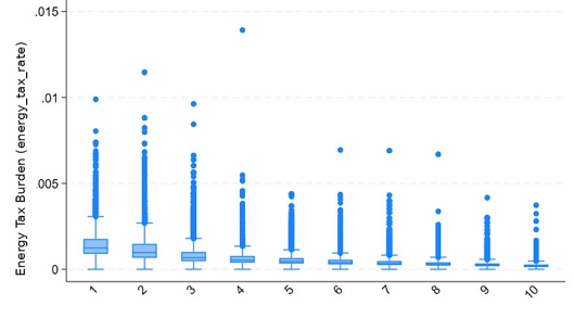
Distribution of the energy tax burden by income decileNote: The figure presents the distribution of the household energy tax burden across income deciles. The energy tax burden is measured as the estimated energy-related tax payment divided by household income.
From a climate policy perspective, the descriptive results indicate that the distribution of household burdens should be examined alongside aggregate environmental or fiscal indicators. Energy taxation may work as a price-based climate policy instrument, but its incidence across income groups is relevant for assessing policy fairness and acceptability.
4.2. Declining average burden and persistent distributional differences
Fig. 2 shows a downward trend in the average household energy tax burden over the sample period. This aggregate decline may reflect changes in household income, energy consumption, energy prices, tax components, or broader economic conditions. Because the dependent variable is expressed as a share of household income, changes in both the numerator and the denominator can affect the observed trend.
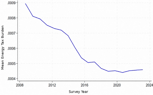
Trend in the average household energy tax burden, 2008–2024Note: The figure reports the annual average of the household energy tax burden over the sample period. The energy tax burden is calculated as estimated energy-related tax payments divided by household income.
The decline in the average burden does not remove the cross-income pattern shown in Table 2. Lower-income households still record higher relative burdens than higher-income households. This distinction is important for the empirical strategy in Section 4: aggregate trends are controlled through year effects, while the income-decile coefficients identify differences in the burden across relative income positions after accounting for common annual shocks.
Appendix Fig. A1 presents the corresponding trends for the 1st, 2nd, and 5th income deciles. All three groups show a broad decline over the sample period, while their relative ordering remains stable, with the 1st decile recording the highest average burden, followed by the 2nd and 5th deciles. These persistent differences indicate that the aggregate decline shown in Fig. 2 did not eliminate the relative burden gaps across the selected income groups.
4.3. Income gradient in the panel regression results
Table 3 reports the pooled OLS, fixed-effects, and random-effects estimates from the baseline specification. In all three models, the coefficients for the higher income deciles are negative and statistically significant. Since the 1st income decile is the reference group, these coefficients indicate that households in higher income groups have lower energy tax burdens than households in the lowest income group after accounting for survey-wave effects. Additional controlled specifications are reported in Appendix Table A2.
Panel regression results for energy tax burden per 10,000 KRW of income
The fixed-effects estimates are used as the main specification because they control for unobserved, time-invariant household characteristics. After rescaling the dependent variable in Table 3, the coefficient for the 2nd decile is -3.5090, while the coefficient for the 10th decile is -13.2990. These estimates indicate that higher-income households bear a lower energy tax burden per 10,000 KRW of household income than households in the lowest income decile. The estimates therefore support a systematic income gradient in the household energy tax burden. This finding is consistent with the descriptive evidence, but it is stronger in the sense that it remains after controlling for household fixed effects and survey-wave effects.
The controlled robustness estimates in Appendix Table A2 show that the negative and generally monotonic income gradient remains after adding household size, a household-head age proxy, and regional indicators. In the fixed-effects specification, the coefficient is -3.5619 for the 2nd decile and -13.9212 for the 10th decile, and both are statistically significant at the 1% level. The random-effects estimates in this controlled specification also lie between the pooled OLS and fixed-effects estimates across the income deciles. Thus, the substantive conclusion that relative energy tax burdens decline as income rises is robust to the inclusion of these observed household and regional characteristics.
The similarity of the coefficient signs across pooled OLS, fixed-effects, and random-effects models indicates that the negative income gradient is not driven by a single model choice. At the same time, the fixed-effects estimates should be interpreted as within-household associations rather than as evidence of a fully causal effect of income mobility on the energy tax burden. The estimates show that, conditional on the empirical specification, households in higher income deciles face lower relative energy tax burdens than households in the lowest decile.
4.4. Association between general public transfer receipt and the energy tax burden
Table 4 examines whether income-decile differences in the household energy tax burden vary by the general public transfer indicator defined in Section 3.3. Because the indicator combines multiple broad transfer categories, the estimates are interpreted as conditional associations with general public transfer receipt rather than as the direct effect of a dedicated energy-tax rebate, revenue-recycling scheme, or specific Korean energy-welfare program.
Association between general public transfer receipt and energy tax burden per 10,000 KRW of income
Appendix Table A3 shows that 31.3% of the panel observations received at least one form of general public transfer. Receipt rates range from 25.8% in the 10th income decile to 35.0% in the 6th decile and are not strictly monotonic across the income distribution. This pattern reflects the broad construction of the indicator, which combines support linked to age, household circumstances, temporary shocks, and economic need rather than a single income-tested energy-compensation program. The interaction estimates should therefore be interpreted in light of this heterogeneous recipient composition.
The interaction term is negative and statistically significant for the 2nd decile. Because the income-decile effect is already negative, the additional negative interaction indicates that the difference between the 2nd and 1st income deciles is more negative among general public transfer recipients than among non-recipients. The interaction terms for the 3rd and 4th deciles are also negative but are not statistically significant, while the positive interaction for the 5th decile is likewise not statistically significant. From the 6th decile onward, the interaction terms are positive and statistically significant, indicating that the negative income-decile differences are modestly narrower among general public transfer recipients than among non-recipients. The calculated combined differences remain negative across all income deciles, indicating that the underlying income gradient persists among observations receiving general public transfers.
These results do not show a uniform moderating association between general public transfer receipt and the income gradient. Among transfer recipients, the difference between the 2nd and 1st income deciles is wider than among non-recipients, whereas the differences for the 3rd–5th deciles are not statistically distinguishable across transfer-receipt status. For the 6th–10th deciles, the negative income-decile differences are modestly narrower among transfer recipients. Overall, the association varies across income groups, while the underlying income gradient remains present. Because the combined difference is the sum of the income-decile effect and the interaction term, it represents the remaining income-decile difference among transfer recipients rather than the absolute burden level or the causal effect of receiving support. These estimates do not imply that Korea’s Energy Voucher Program, utility tariff reductions, or other specific energy-welfare measures are ineffective. Evaluating those programs would require program-specific information on eligibility, participation, benefit amounts, and the timing of receipt.
4.5. Distributional heterogeneity across the tax burden distribution
Table 5 reports conditional quantile regression estimates for the 10th income decile at 0.25, 0.50, and 0.75 quantiles. As in Tables 3 and 4, the dependent variable is rescaled by multiplying the original household energy tax burden ratio by 10,000. The coefficient is negative and statistically significant at all three quantiles. The estimated coefficient is -8.0580 at the 0.25 quantile, -10.9300 at the median, and -15.3960 at the 0.75 quantile. This pattern suggests that the difference between the 10th and 1st income deciles is larger at higher points of the conditional distribution of the energy tax burden.
Conditional quantile regression results for energy tax burden per 10,000 KRW of income
Fig. 3 provides a visual summary of the quantile regression results. The estimated coefficients become more negative as income deciles rise, and the slope is steeper at the upper quantile. This suggests that the regressive pattern is not confined to the mean relationship. It is also observed across the conditional distribution and appears more pronounced among households with higher relative energy tax burdens. The result should be understood as evidence of distributional heterogeneity rather than as a direct test of the mechanisms behind high burden levels.
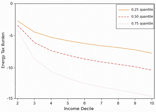
Quantile regression coefficients by income decileNote: The figure plots the estimated coefficients across income deciles at the 0.25, 0.50, and 0.75 quantiles. The dependent variable is the household energy tax burden rescaled by multiplying the original burden ratio by 10,000. The 1st income decile is the reference group.
4.6. Discussion of the main findings and policy relevance
Because household income is both the denominator of the burden measure and the basis for assigning income deciles, a negative association between income position and the burden ratio is partly expected by construction. This feature means that the contribution of the analysis cannot rest on the sign of the income gradient alone. The empirical contribution lies in documenting how large the gradient is, whether it reflects only comparisons between unlike households, whether it remains after controlling for time-invariant household heterogeneity and common annual shocks, and whether it varies across the burden distribution. The fixed-effects estimates remain associational and do not remove the arithmetic role of income in the denominator.
Appendix Table A4 shows that the mean estimated annual energy-related tax payment rises from KRW 212,088 in the 1st income decile to KRW 349,272 in the 10th decile. Higher-income households therefore make larger estimated annual payments in absolute terms. Nevertheless, Table 2 shows that the payment-to-income ratio falls from 0.0014 in the 1st decile to 0.0002 in the 10th decile. Taken together, these results indicate that absolute estimated annual payments are higher among higher-income households, whereas the relative burden is substantially higher among lower-income households. The regressivity documented here does not arise because lower-income households make larger absolute payments; rather, estimated annual payments increase much less than proportionately with household income across the income distribution.
Tables 2 and 3 also distinguish the descriptive pattern from a persistent panel association. Using the rounded means in Table 2, the difference between the 1st and 10th deciles is approximately 12 units per 10,000 of household income. The corresponding 10th-decile coefficients in Table 3 are -13.2780 in pooled OLS and -13.2990 in the household fixed-effects model. Although the descriptive and regression figures are not exactly identical because of rounding and the inclusion of survey-wave effects, their similar magnitude shows that controlling for time-invariant household characteristics and common annual shocks does not explain away the income gradient. In other words, within the same households over time, movement to a higher relative income position is associated with a lower relative energy tax burden. Appendix Table A2 further shows that this conclusion remains when household size, the household-head age proxy, and regional indicators are added.
The conditional quantile results provide an additional contribution beyond the mean comparison. The estimated difference between the 10th and 1st deciles increases in magnitude from -8.0580 at the 0.25 quantile to -10.9300 at the median and -15.3960 at the 0.75 quantile. The regressive income gradient is therefore stronger among households located at higher points of the burden distribution. This finding indicates that income alone does not fully identify energy vulnerability: households with similar income positions may face different burdens because of housing efficiency, heating and cooling needs, transportation dependence, household composition, or access to substitutes. The result provides an empirical basis for considering actual relative energy burden as a supplementary targeting criterion alongside income.
The findings for general public transfers have a more limited policy interpretation. Table 4 and Appendix Table A3 show that the indicator covers heterogeneous transfers and that receipt is not monotonically concentrated in the lowest income deciles. The interaction results do not reveal a uniform moderating pattern. Among general public transfer recipients, the difference between the 2nd and 1st income deciles is wider than among non-recipients, the differences for the 3rd–5th deciles are not statistically distinguishable by transfer-receipt status, and the negative differences for the 6th–10th deciles are modestly narrower. The underlying income gradient nevertheless remains present among transfer recipients. As discussed in Section 2.3, broad public transfers are distinct from Korea’s existing energy-affordability measures and from dedicated energy-tax compensation financed through revenue recycling. The heterogeneous interaction pattern therefore reinforces the need to distinguish general public transfers from compensation instruments specifically designed around energy-tax exposure. The results support two cautious design principles: protection should be sensitive to household income, and it may be improved by considering actual energy burden. They do not establish that any existing Korean energy-support program is ineffective, nor do they identify the optimal form or amount of compensation; those questions require program-specific data.
4.7. Limitations and scope for future research
First, the estimated energy-related tax payment is a standardized expenditure-based measure rather than an administrative record of household-specific tax liabilities. Broad expenditure categories and standardized rates do not separately identify physical consumption, unit prices, tax pass-through, or local and temporal differences in effective incidence. Accordingly, the reported income-decile gaps should be interpreted as comparative estimates under a common construction rather than as exact differences in observed tax payments.
Second, the fixed-effects design controls for unobserved household characteristics that remain constant over time, but it cannot remove all time-varying confounding. Household employment, health, composition, housing conditions, and localized weather may change jointly with income position and energy demand. The estimates therefore establish persistent conditional associations and distributional heterogeneity, not a causal mechanism through which income mobility changes energy-tax incidence.
Finally, the analysis is retrospective and is not designed to forecast household responses to a future explicit carbon tax. The estimates describe the historical incidence of a standardized energy-related tax burden through 2024, but they do not identify energy-demand elasticities, behavioral adaptation, welfare changes, or the effects of alternative revenue-recycling arrangements. Future research could combine administrative tax or utility-billing microdata with program-specific transfer records and dynamic microsimulation or computable general equilibrium models. Such extensions would allow explicit comparison of lump-sum rebates, income-targeted compensation, energy-voucher expansion, and residential efficiency investment under alternative carbon-pricing scenarios.
5. Conclusion
This study examined the distributional implications of energy taxation in Korea using household-level panel data from the National Survey of Tax and Benefit for 2008–2024. Its contribution is not simply to report the expected negative relationship between income and a burden measure that uses income as its denominator. Rather, it shows that the regressive gradient is substantial in magnitude, persists after household fixed effects and survey-wave effects are introduced, becomes stronger at higher points of the burden distribution, and remains present among general public transfer recipients despite heterogeneous differences in the gradient across income groups.
The comparison of absolute payments and relative burdens is central to this interpretation. Higher-income households make larger estimated energy-related tax payments in absolute terms, but the increase in payments is much smaller than the increase in household income. Consequently, lower-income households devote a substantially larger share of income to the estimated burden. The fixed-effects estimate for the 10th decile is close in magnitude to the descriptive gap between the lowest and highest deciles, indicating that the pattern is not solely attributable to cross-sectional differences between households. The quantile results further show that the gap between low- and high-income households is largest among households already facing relatively high burdens.
The policy implications follow directly from these results but should be interpreted as design principles rather than as calibrated recommendations. First, the findings provide an empirical rationale for considering household income as a central targeting criterion in the design of future compensation associated with energy taxation or carbon pricing, so that the environmental price signal can be maintained without imposing disproportionate relative burdens on low-income households. Second, the quantile results provide a rationale for examining whether an indicator of actual relative energy burden could supplement income-based eligibility. Korea’s Energy Voucher Program, electricity and gas tariff reductions, and low-income household energy-efficiency support provide existing administrative channels for addressing energy vulnerability, but these energy-affordability measures should not be equated with dedicated recycling of energy-tax revenues. Likewise, the general public transfer indicator used in this study is broader than those programs. Its association with the burden gradient is heterogeneous across income groups and does not show a uniform moderating pattern. This finding cannot be interpreted as evidence that any specific energy-welfare measure is ineffective. The analysis does not calibrate eligibility thresholds, benefit amounts, or fiscal costs.
Several limitations define the scope of these conclusions. The energy-related tax payment is estimated from household expenditures and standardized indirect tax rates rather than observed in administrative tax records. Because household income is included in the denominator and used to construct income deciles, part of the negative gradient is mechanical, although the comparison with absolute payments, the panel estimates, and the quantile results provides evidence beyond the sign alone. Household fixed effects also do not eliminate time-varying household or local shocks, so the estimates should not be interpreted causally. In addition, the broad transfer indicator does not identify individual programs, benefit amounts, or eligibility rules. Finally, the retrospective analysis through 2024 does not predict behavioral, welfare, or revenue-recycling effects under a future explicit carbon tax. Future research using administrative tax or utility-billing data, program-specific transfer records, and dynamic microsimulation or general equilibrium models would allow more direct evaluation of these policy pathways.
Acknowledgments
An earlier version of this paper was presented at the 2025 KIPF National Survey of Tax and Benefit (NASTAB) Conference. This revised version has been substantially updated and expanded. The author gratefully acknowledges the Korea Institute of Public Finance (KIPF) for providing the NASTAB panel data.
References
-
Amores AF, Maier S, Ricci M. 2023. Taxing household energy consumption in the EU: The tax burden and its redistributive effect. Energy Policy 182: 113721.
[https://doi.org/10.1016/j.enpol.2023.113721]

- Burke J, Fankhauser S, Kazaglis A, Kessler L, Khandelwal N, Bolk J, Owen A. 2020. Distributional impacts of a carbon tax in the UK. London: Grantham Research Institute on Climate Change and the Environment.
-
Carattini S, Carvalho M, Fankhauser S. 2018. Overcoming public resistance to carbon taxes. WIREs Clim Change 9(5): e531.
[https://doi.org/10.1002/wcc.531]
-
Cronin JA, Fullerton D, Sexton S. 2019. Vertical and horizontal redistributions from a carbon tax and rebate. J Assoc Environ Resour Econ 6(S1): S169-S208.
[https://doi.org/10.1086/701191]
-
Dechezleprêtre A, Fabre A, Kruse T, Planterose B, Sanchez Chico A, Stantcheva S. 2025. Fighting climate change: International attitudes toward climate policies. Am Econ Rev 115(4): 1258-1300.
[https://doi.org/10.1257/aer.20230501]
-
Dorband II, Jakob M, Kalkuhl M, Steckel JC. 2019. Poverty and distributional effects of carbon pricing in low- and middle-income countries: A global comparative analysis. World Dev 115: 246-257.
[https://doi.org/10.1016/j.worlddev.2018.11.015]
-
Douenne T, Fabre A. 2022. Yellow vests, pessimistic beliefs, and carbon tax aversion. Am Econ J Econ Policy 14(1): 81-110.
[https://doi.org/10.1257/pol.20200092]
-
Goulder LH, Parry IWH. 2008. Instrument choice in environmental policy. Rev Environ Econ Policy 2(2): 152-174.
[https://doi.org/10.1093/reep/ren005]
-
Grainger CA, Kolstad CD. 2010. Who pays a price on carbon? Environ Resour Econ 46(3): 359-376.
[https://doi.org/10.1007/s10640-010-9345-x]
-
Hassett KA, Mathur A, Metcalf GE. 2009. The incidence of a U.S. carbon tax: A lifetime and regional analysis. Energy J 30(2): 155-177.
[https://doi.org/10.5547/ISSN0195-6574-EJ-Vol30-No2-8]
-
Klenert D, Mattauch L, Combet E, Edenhofer O, Hepburn C, Rafaty R, Stern N. 2018. Making carbon pricing work for citizens. Nat Clim Chang 8(8): 669-677.
[https://doi.org/10.1038/s41558-018-0201-2]
- Korea Electric Power Corporation. 2026. Welfare discount guide. Naju: Korea Electric Power Corporation; [accessed 2026 Jul 16]. Available from: https://online.kepco.co.kr/MIM021D00
- Korea Energy Agency. 2026. Energy voucher program: Support information. Ulsan: Korea Energy Agency; [accessed 2026 Jul 16]. Available from: https://www.energyv.or.kr/info/support_info.do
- Korea Energy Foundation. 2026. Low-income household energy-efficiency improvement program. Seoul: Korea Energy Foundation; [accessed 2026 Jul 16]. Available from: https://e-welfare.koref.or.kr/introduce
- Korea Gas Corporation. 2026. Energy welfare program: Gas tariff reductions for socially vulnerable customers. Daegu: Korea Gas Corporation; [accessed 2026 Jul 16]. Available from: https://www.kogas.or.kr/site/koGas/1020408010000
- Lee J, Kim W. 2022. Effects of carbon taxation on household welfare and CO2 emission. Korean Energy Econ Rev 21(2): 33-74.
-
Metcalf GE. 2009. Market-based policy options to control U.S. greenhouse gas emissions. J Econ Perspect 23(2): 5-27.
[https://doi.org/10.1257/jep.23.2.5]
-
Mildenberger M, Lachapelle E, Harrison K, Stadelmann-Steffen I. 2022. Limited impacts of carbon tax rebate programmes on public support for carbon pricing. Nat Clim Change 12: 141-147.
[https://doi.org/10.1038/s41558-021-01268-3]
- OECD. 2015. The distributional effects of energy taxes. Paris: OECD Publishing.
-
Pizer WA, Sexton S. 2019. The distributional impacts of energy taxes. Rev Environ Econ Policy 13(1): 104-123.
[https://doi.org/10.1093/reep/rey021]
-
Poterba JM. 1991. Is the gas tax regressive? In: Bradford D (ed). Tax policy and the economy, Vol. 5. Cambridge: MIT Press. p. 145-164.
[https://doi.org/10.1086/tpe.5.20061803]
-
Rausch S, Metcalf GE, Reilly JM. 2011. Distributional impacts of carbon pricing: A general equilibrium approach with micro-data for households. Energy Econ 33(Suppl 1): S20-S33.
[https://doi.org/10.1016/j.eneco.2011.07.023]
-
Williams RC III, Gordon H, Burtraw D, Carbone JC, Morgenstern RD. 2015. The initial incidence of a carbon tax across income groups. Natl Tax J 68(1): 195-214.
[https://doi.org/10.17310/ntj.2015.1.09]
- Yi D, Kim SR. 2017. The distributional effects of energy taxes in Korea. Seoul: Korea Institute of Public Finance.
Appendix
Appendix
Energy expenditure categories and applied indirect tax rates
Controlled robustness results
Mean general public transfer receipt indicator by income decile
Descriptive statistics of estimated energy-related tax payments by income decile
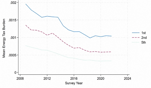
Trends in the average household energy tax burden for the 1st, 2nd, and 5th income decilesNote: The figure reports the annual average household energy tax burden for the 1st, 2nd, and 5th income deciles over the sample period, 2008–2024. The household energy tax burden is measured as estimated annual energy-related tax payments divided by annual household income.